pyradiobiology is a package for radiobiological modeling (TCP, NTCP, EUD, gEUD) with Python.

It provides:

• Linear quadratic model for survival fraction and biological effective dose calculation
• Tumor Control Probability (TCP) models: linear-quadratic Poisson, empirical Poisson
• Normal Tissue Complication Probability (NTCP) model: Relative seriality (RS), Lyman-Kutcher-Burman (LKB)
• Generalized Equi-effective Uniform Dose (gEUD), Equi-effective Uniform Dose (EUD)

To install the package, just run:

pip install pyradiobiology

TcpEmpirical model

The TCP emipirical model or linear-quadratic Poisson model is given by:

\( P(D) = P(EQD_{2Gy}) = exp(-e^{eγ – (EQD_{2Gy}/D_{50})*(eγ-lnln2)}) \)

\(P(D)\) is the tumour control probability, when the tumour is homogenously irradiated at the total dose D and \(EQD_{2Gy}\) is the equi-effective dose at 2Gy per fraction of the total dose D when delivered at a fraction dose d.

\(\bf{D_{50}}\) is the dose in Gy, defined as EQD2, which results in a TCP value of 50% and \(\bf{γ}\) is a dimensionless parameter, defining the maximum normalized value of the dose-response gradient.

For an inhomogeneous dose distribution {D} within the tumour of volume V, the overall tumour control probability TCP is calculated according to:

\( TCP({D},V) = \prod_{i=1}^N[P(D_{i})]^{v_{i}/V} \)

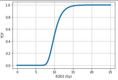
Now, let’s plot the TCP for a homogeneous dose distribution with pyRadiobiology:

from pyradiobiology import * 
import matplotlib.pyplot as plt
import numpy as np

doses = DoseBag(data=[*np.arange(start=0, stop=25, step=0.01)], 
                  unit=DoseUnit.GY, 
                  dose_type=DoseType.EQD2)

 
model = TcpEmpirical(d50=Dose.gy(10, DoseType.EQD2),
                     gamma=2.63)

tcp_voxels = model.voxel_response(doses)
plt.plot(doses.data, tcp_voxels, linewidth=4)
plt.xlabel("EQD2 (Gy)")
plt.ylabel("TCP")
plt.grid()
plt.show()

The output:

The TCP calculation for an inhomogeneous dose distribution can be performed as follows. Here, we have a tumor with two regions of 15 cc and 20 cc. The regions receive 70 Gy and 65 Gy, respectively. Further, assumptions are \( α/β = 3.0 Gy \) and the number of fractions, nfx = 40.

from pyradiobiology import * 
tcpmodel = TcpEmpirical(
    d50=Dose.gy(55, dose_type=DoseType.EQD2), 
    gamma=6.7)
dose_array = DoseBag.create(data=[70, 65], 
                            unit=DoseUnit.GY,
                            dose_type=DoseType.PHYSICAL_DOSE)
volume_array_in_cc = [15, 20]
tcp = tcpmodel.response_from_pysical_dose(
                                dose_array_in_physical_dose=dose_array,
                                volume_array=volume_array_in_cc,
                                ab_ratio=Dose.gy(3.0),
                                nfx=40)
 print(f"from physical dose, calculated TCP = {round(tcp, 4)}")
#self.assertEqual(0.9266, round(tcp, 4))

So, in the above example you can also use the (dose, volume) tuples/pairs derived by a differential Dose-Volume-Histogram (DDVH).