A CVT is a special type of Voronoi tessellation when each generator, of each Voronoi cell, is located in the center of the mass of the cell.  CVT is an optimal partition corresponding to an optimal distribution of generators.

A set \(\Omega \subseteq \mathbb{R}^n\) is tessellated by k generators \(z_i\) (is the position of the generator) into k Voronoi cells \(V_i\) (denoting the Euclidean distance):

Every element x in the Ω set is exactly assigned to one Voronoi cell. The distance from an element x to the generator \(z_i\) of the corresponding Voronoi cell is always shorter than to any other generators

A density ρ(x) can be defined on the Ω set. Every point x in Vi has a density value assigned. The center of mass (or centroid) \(z_i^*\) for a Voronoi is defined by:

A Voronoi tessellation is called a centroidal Voronoi tessellation (CVT) if the generators zi are also the centers of mass) \(z_i^*\) of their Voronoi region. An algorithm to calculate the CVT is the iterative Lloyd’s algorithm. The energy- (also cost-, distortion-error- or variance-) function is calculated by:

The CVT minimizes the energy function and can, therefore, be determined by calculating the global minimum of the energy function.

Lloyd’s Algorithm is a method for finding the centroidal Voronoi diagrams for a given region Ω and density function ρ(x, y). In Lloyd’s algorithm, an initial Voronoi diagram is made with the desired number of generators over the region Ω. Then, the centroids of the Voronoi regions are computed and a new Voronoi diagram is created using the centroids as the generator points. This is repeated for a given number of iterations or until some stopping criterion on the new generators are met.

The following is a more precise algorithm as stated in Probabilistic Methods for Centroidal Voronoi Tessellations and Their Parallel Implementations [1]:

Given a region Ω, and density function ρ(x) defined for all x ∈ Ω, and a positive integer k:

(1) Choose an initial set of k points \({z_i}\)  with  \(  i=1..k\) in Ω, e.g., by using a Monte Carlo method.

(2) Construct the Voronoi sets \({V_i}\)  with  \( i=1..k\) associated with \({z_i}\)  with \(i=1..k \).

(3) Determine the mass centroids of the Voronoi sets \({V_i}\)  with  \(i=1..k\) these centroids form the new set of points \({z_i}\)  with   \(i=1..k \).

(4) If the new points meet some convergence criterion, terminate; otherwise, return to step 2.

Space partitioning of a prostate structure

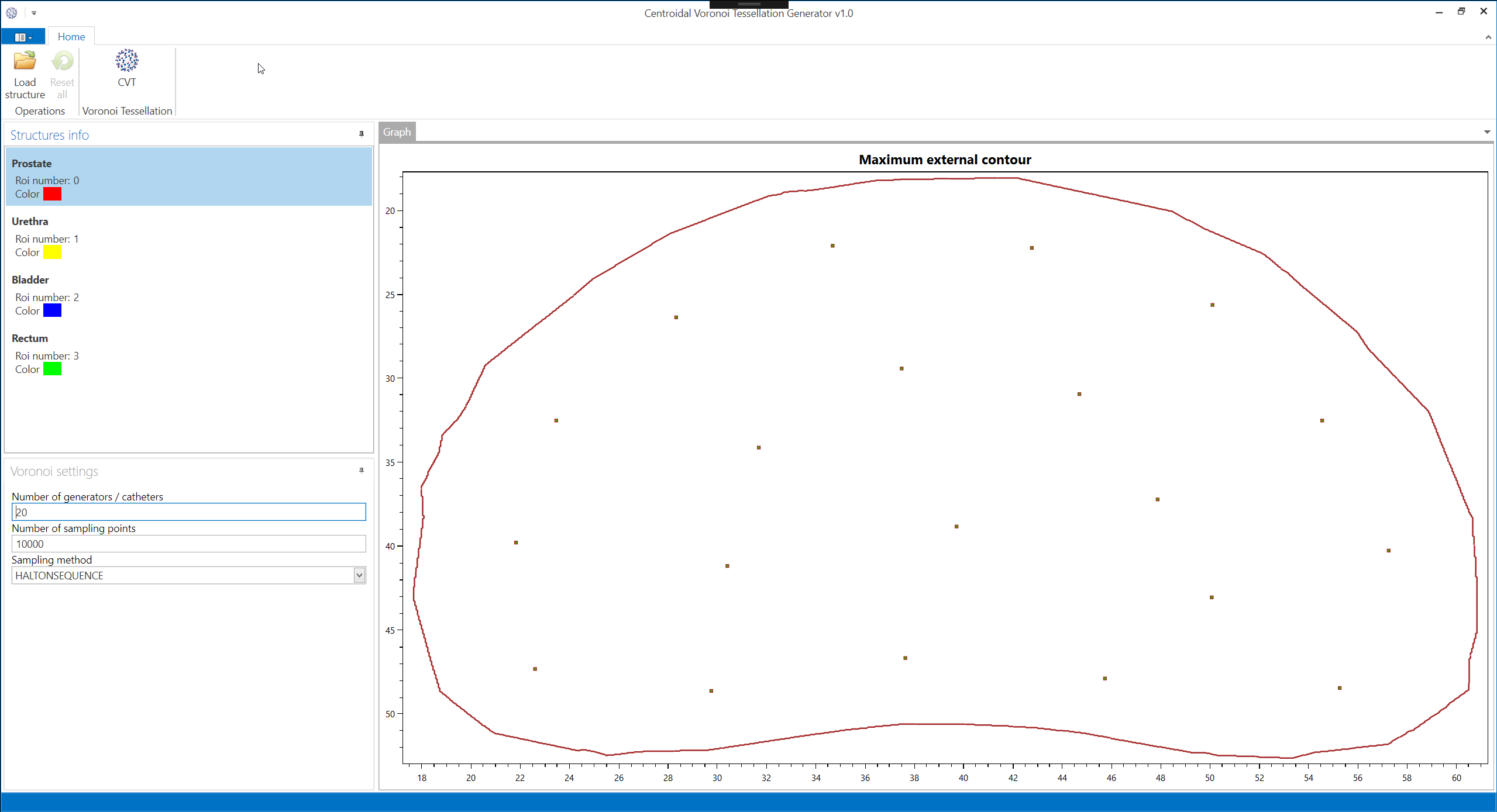
A testing application can be downloaded from: https://github.com/isachpaz/CVTGenerator

Related publication:

Sachpazidis, Ilias; Hense, Jürgen; Mavroidis, Panayiotis; Gainey, Mark; Baltas, Dimos “Investigating the role of constrained CVT and CVT in HIPO inverse planning for HDR brachytherapy of prostate cancer“, Journal Article Medical Physics Journal, 2019, https://aapm.onlinelibrary.wiley.com/doi/10.1002/mp.13564 

References

[1] Du, Qiang, Vance Faber, and Max Gunzburger. Centroidal Voronoi Tessellations: Applications and Algorithms. Society for Industrial and Applied Mathematics. (1999): 637-676.